How we built a web-scale vector database

The problem
At Exa, we're redesigning web search from scratch to handle complex queries that Google can't. To do that, we needed to build our own web-scale vector database.
In this blog post, we'll describe in detail how that vector database works—from high-level algorithms, to low-level optimizations that we haven't seen in existing literature.
The end result is a database that can search billions of vectors in under 100ms with high recall, all while enabling keyword + metadata filters and using less memory than a gaming PC.
The Challenge
Exa needs to handle complex semantic queries like "AI startups in the Bay Area building hardware" and return a list of companies that exactly match that criteria.
To capture the semantic meaning of a document, we convert the document into a vector (aka an embedding). Documents with similar meanings become embeddings with similar numerical values.
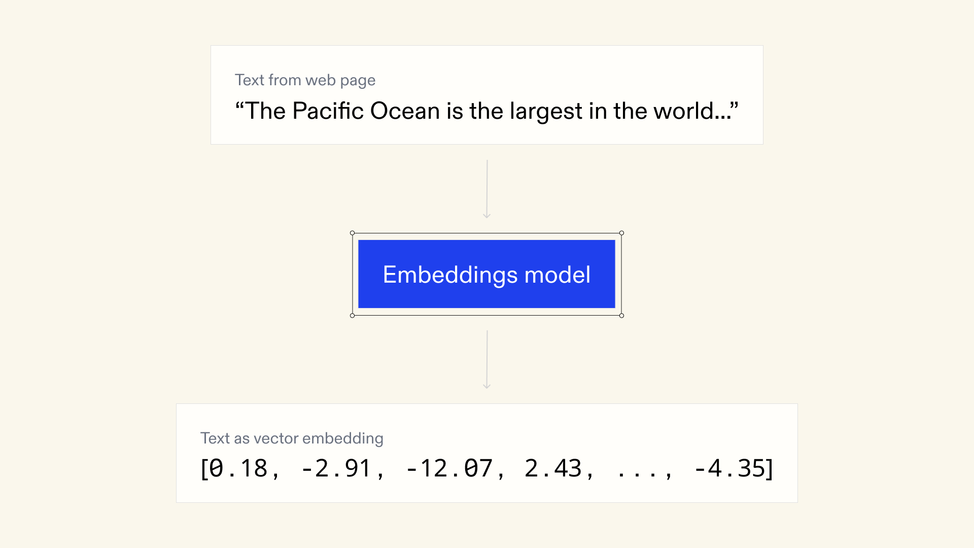
To search through the documents, we convert the user's query into an embedding, compare it against the embeddings of all the web documents we've indexed, and return the closest matches.
So, we need to store all our document embeddings in a way that's memory-efficient and enables fast search, without losing precision.
Our Engineering Requirements
- Search billions of vectors, each of which consists of 4096 floating-point numbers.
- Handle metadata filtering efficiently — e.g., only return documents between 2022 and 2023, or from reddit.com and youtube.com
- Return search results in under 100 ms.
- Handle >500 queries per second at reasonable cost.
Exa's approach
We combined five optimizations to significantly improve memory usage and speed.
Optimization 1: Approximate the embedding
Turns out, you can take any of these 4096-dimensional embeddings, chop off everything except the first 256 elements, and retain much of its meaning.
How? We trained our embeddings model—i.e., the algorithm that transforms raw web pages into their vector representations—using Matryoshka.[1]
Matryoshka is a technique that forces prefixes of embeddings to be approximations of the whole embedding. Meaning: the first 2048 dimensions are a good embedding, the first 1024 dimensions are also a good embedding, etc— down to, say, the first 32 dimensions.
We cut our vectors to 256 dimensions, which reduced memory usage by 20x.
Optimization 2: Compress each dimension
Now each embedding comprises 256 floating-point numbers, but that's still too slow to fully search through.
How can we speed it up?
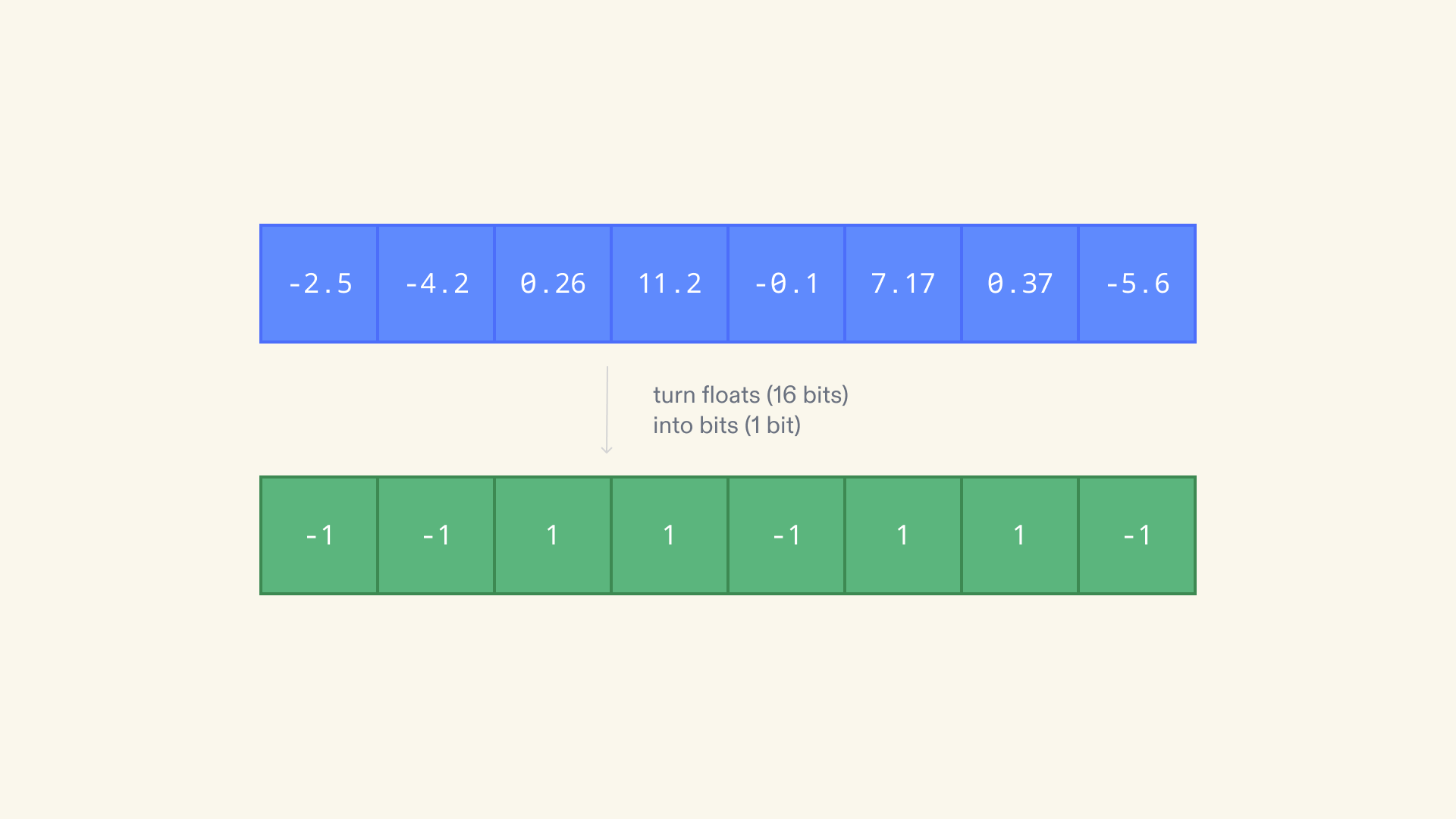
Well, each of these floats occupies 16 bits of space. We used binary quantization to replace the 16-bit floats with 1-bit values. For each float in the vector: if it's greater than 0, set it to 1; else, set it to -1.
This cut our memory usage another 16 times!
Optimization 3: Dot-product optimization
The standard search method for binary-quantized embeddings is to compute the Hamming distance (i.e. number of elements that are different) from the binary-quantized query embedding to each binary document vector.
But this was lossy and inefficient. So we developed a novel hybrid approach: Keep using binary document embeddings—but for the query embedding, use uncompressed floating-points.
Then use dot product as a similarity metric between the query vector and each of the binary-quantized document vectors. (Imagine two vectors in geometric space—the dot product measures the angle between them. A large dot product means the vectors are pointing in the same direction and thus very similar.)
We hyper-optimized our dot product calculations with a strange but effective method:
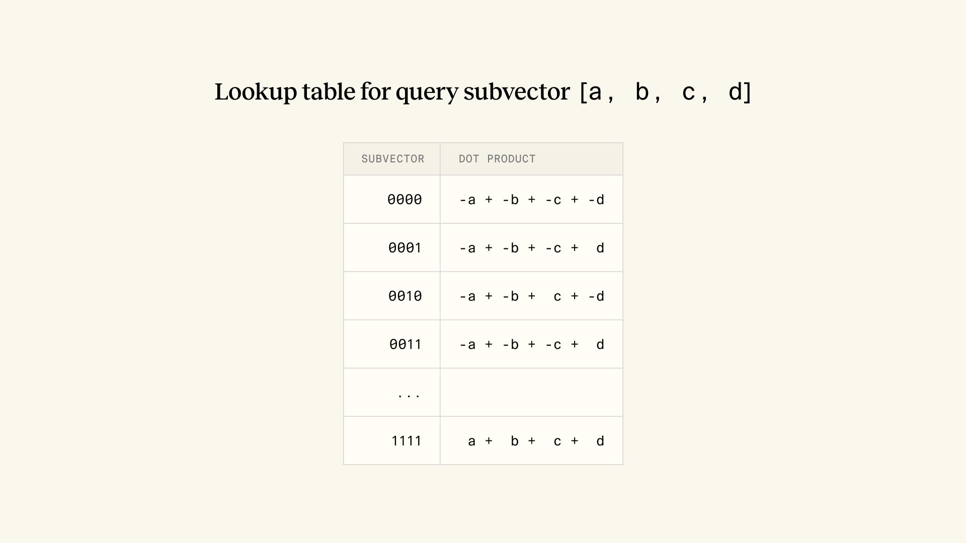
- You can compute the dot product of two vectors by dividing them into smaller subvectors (e.g., of length 4), calculating the dot products of corresponding subvectors, and summing the results.
- Remember: each value in the document vector is either -1 or 1. So any length-4 subvector of a document vector can only have one of 16 possible values. For each length-4 subvector of the query vector, we precompute all 16 possible dot products that it could have with any document subvector, and store those in a lookup table.
- To compute a query-document dot product, we break the document into subvectors, look up each subvector's dot product in the table, and sum them.
This cuts down the number of computations by 1/4.[2]
Optimization 4: Max out the hardware
We further optimized lookup times by loading the entire lookup table into CPU registers. This enables much faster lookups than keeping it in RAM.[3]
Optimization 5: Don't search through everything
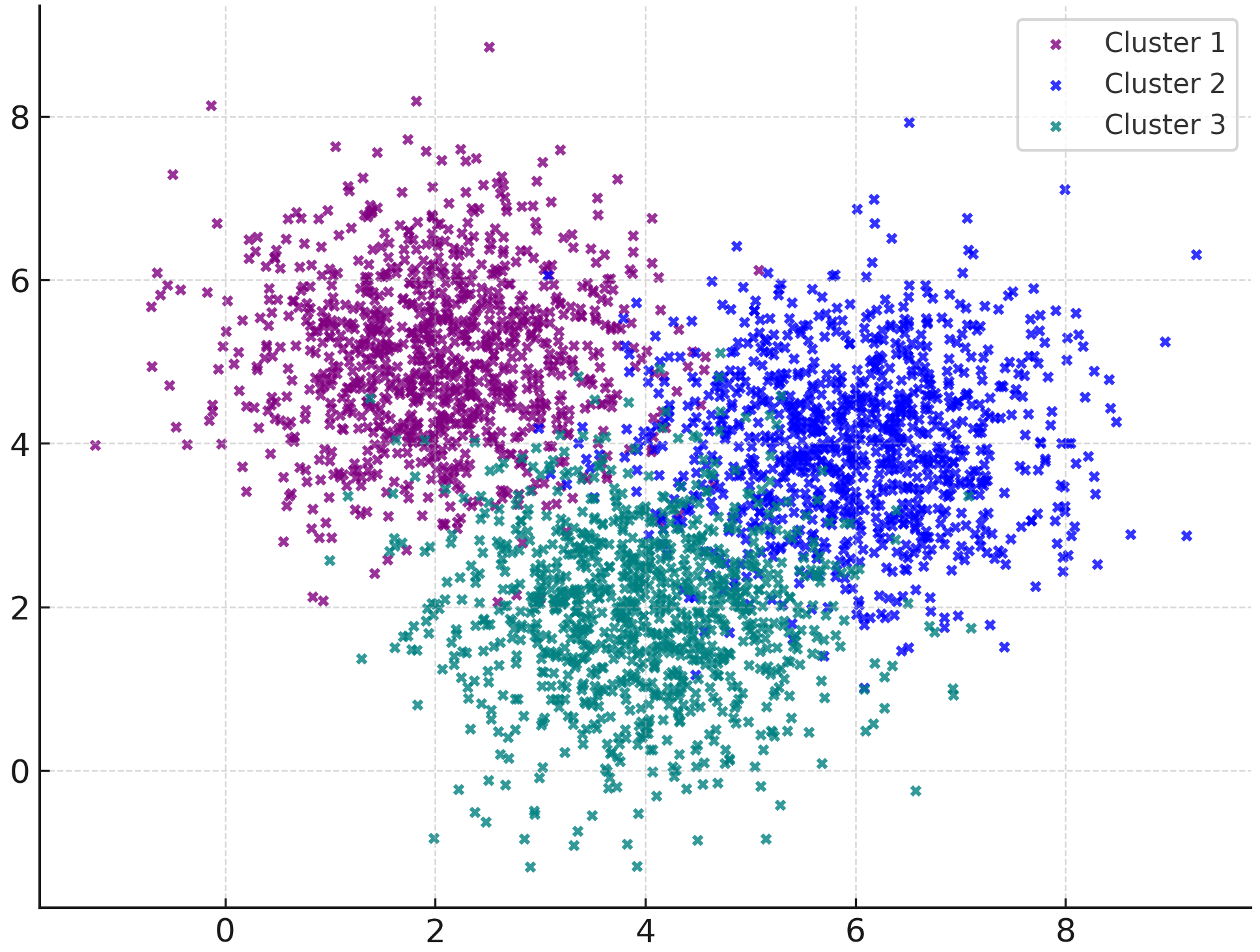
Thus far, we've still been looking through every document embedding on every search. Clustering fixes that.
We divided our documents into 100,000 clusters, each grouped by similarity. When we search, we figure out which cluster our query embedding belongs in, and only search through that cluster and nearby ones.
With clustering, we can get a roughly 1000x improvement in throughput without much accuracy degradation 🤯.
Final touches
Recovering recall
You might wonder—haven't we just cut out a lot of information by truncating and squashing the vectors so aggressively?
Yes, these optimizations are lossy. But nothing some reranking can't fix. After the initial search, we fetch extra results and rerank them with the uncompressed data.
Filtering
We deliberately designed the vector database to allow for complex filters, like filtering by date range, domain, or keyword. Basically we want our vector database to act like a database!
Unlike graph-based methods like HNSW, our clustering compressed methods fit nicely with filters. For each filterable value (category, date, etc), we create inverted indexes. These are hashmaps from the filterable value to a list of document IDs that match the filter. If the user specifies a filter, then we only run our search algorithm over the documents that match the filter in the inverted index.
Final system
- We cut costs 10x compared to quotes from cloud vector database services.
- We can shard our data more easily (e.g. by cluster) than HNSW (whose global graph structure can't be partitioned easily).
- We can add filters for our data more efficiently.
- We can build fun custom solutions on top of it. E.g. We built our own query language that allows us to easily define different multi-stage pipelines for different scoring algorithms.
This is only the beginning. Turns out a standard vector database is not enough for perfect web search. More coming there :)
P.S. If this post left you hungry for more, come help us fix web search.

